Vérification des Dépendances R

Introduction

Ce document est un exemple de fichier Quarto Markdown (.qmd) qui utilise R, Jupyter, et d’autres dépendances R.

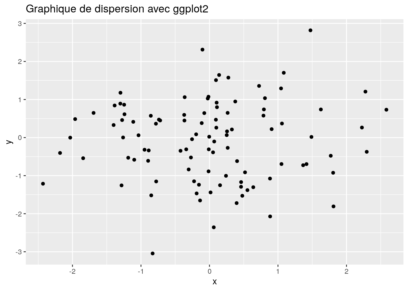
library(knitr)
library(ggplot2)


# Créer un exemple de données
data <- data.frame(
  x = rnorm(100),
  y = rnorm(100)
)

# Créer un graphique de dispersion
plot <- ggplot(data, aes(x = x, y = y)) +
  geom_point() +
  ggtitle("Graphique de dispersion avec ggplot2")

# Afficher le graphique
print(plot)

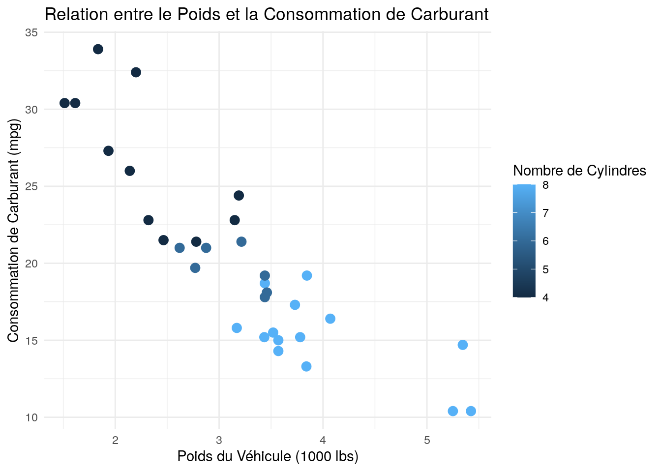
library(ggplot2)
# Charger le jeu de données mtcars
data("mtcars")

# Créer un graphique de dispersion
plot <- ggplot(data = mtcars, aes(x = wt, y = mpg)) +
  geom_point(aes(color = cyl), size = 3) +
  labs(
    title = "Relation entre le Poids et la Consommation de Carburant",
    x = "Poids du Véhicule (1000 lbs)",
    y = "Consommation de Carburant (mpg)",
    color = "Nombre de Cylindres"
  ) +
  theme_minimal()

# Afficher la figure
print(plot)

# Exporter la figure en PNG
ggsave("figure.png", plot = plot, width = 8, height = 6)

# Exporter la figure en PDF
ggsave("figure.pdf", plot = plot, width = 8, height = 6)